A Quick Explanation of Recent NARDL

The News of a positive change  in the character of a villain (did something very good) of your area may surprise you, but his negative change may not.  These two sides of changes do not have an uniform impact on you. Again, think of a very moral person you like. His  negative change may shock you but his positive change won’t. These two changes in opposite directions (positive and negative) do not have the same power to move you, in both examples. And the effects are not really symmetric or equivalent; they are asymmetric or non-equivalent. Asymmetry is one type of non-linearity. The asymmetries and other other forms of non-linearity are also frequent in economic variables. For example, an increase (positive change) in oil price is said to have stronger effect on particular macroeconomic variables than decrease (negative change). In fact, ‘’nonlinearity is endemic within the social sciences and that asymmetry is fundamental to the human condition’’ Shin et al. (2014)

A conventional time series regression model contains constant parameters and assumes that a change in explanatory variable has the same effect over time which may not be appropriate in all cases as shown in the oil example earlier.  Again, the popular cointegration tecniques such as EG-ECM, VECM, Bound testing etc. imply a constant speed of adjustment ( i.e a constant ECT) to long-run equilibrium after a shock (change). But this dos not hold true always when there is market frictions. (see G Dufrénot, V Mignon 2012). Estimating a relationship which possibly has asymmetry with symmetric techniques seems unfair and may leads one to some serious inappropriate  policy conclusions (Enders 2014)). Since the conventiona cointeration test doesn’t allow one to capture the asymmetries in macroeconomic variables. Various techniques have been introduced so far to account this asymmetry, Threshold ECM, Smooth transition regression ECM. Markov-switching ECM etc. But the recent NARDL or Non-linear Autoregressive Model proposed by shin et al (2014) incorporate asymmetries both in the long run and in short run relationships, and at the same time, it captures the asymmetries in the dynamic adjustment.  Moreover,  it allows the regressors of mixed order of I(0) and I(1).

An illustration: If inflation rate rises in a country you may expect that the domestic foods becomes expensive and there will be a tendency to import foods from foreign countries. The relationship is positive. Again if inflation rate falls the consumers find domestic foods cheaper and people reduce buying foreign foods, the food imports decline (positive relationship). Although in both cases the food imports react positively to the inflation rate, are the magnitudes of reactions same in both cases ? maybe not;  maybe food import response more to positive change or otherwise. A time series regression specification with a constant parameter will tell us that the reaction is same in both direction. Here comes the NARDL. NARDL (also other asymmetric regression techniques) explicitly distinguishes the reactions of both directions. 
I denote food import by food_t and inflation rate by INF_t, intercept by C and residuals by U_t. For simplicity, ignore the other regressors that may influence the food import. The simple OLS two-variable model takes the following form:

Foodt=C+βINFt + Ut.

To capture the possible asymmetric effects of inflation on food import NARDL technique decomposes the inflation rate series into two parts 1)partial sum of positive change in inflation rate denoted by INF_t⁺   and 2) partial sum of positive change in inflation rate denoted by INF_t^-   and include both of them as separate regressors in the model and the model becomes:

Foodt=C+β1 INFt+ + β2 INFt - + Ut.

Clearly, this is now a three-variable OLS model. 
If we now represent this equation in (linear) ARDL model proposed by pesaran et. Al (2001) the final model takes the form as show in picture below. The model shown in the picture is the general form of NARDL. (Non linear Autoregressive Distributed Lag Model. See the explanation of each term in the picture below. 

🔍The long run coefficients: We can calculate the long run coefficient of INF⁺_t by dividing the the negative of the coefficient of INF⁺_{t ,} θ⁺    by the coefficient of Food_{t-1 ,}  ρ, and   the the long run coefficient of INF^- _t  by dividing the negative of the coefficient of INF^-_{t ,} θ^-    by the coefficient of Food_{t-1 ,}  ρ

   (-θ⁺  / ρ) and   (-θ^-  / ρ)  are the long run coefficients of of INF_t⁺   and INF_t^-  , respectively.

The summation notation  Σ  implies that NARDL consider inclusion of differenced variables into model upto some lags. For example, in case of  ∆Food_t-1, NARDL considers the incusion of  its first lagged term upto maximum lag you choose, if appropriate. And in case of  ∆INF^-_t it consider the the inclusion of its zero lag (∆INF^-_t itself)  upto the maximum lag you choose, if appropriate.  

🔍Asymmetric Cointegration test:  A long run relationship or cointegration is present if  the joint null hypothesis,

             ρ =θ⁺  =  θ^- =zero is rejected. The critical value are the same critical values for ARDL.  

🔍Testing Symmetry: Clearly, if the long-run coefficients  (-θ⁺  / ρ) and   (-θ^-  / ρ)  are not same then there is asymmetry in the long run. So we test the null hypothesis of  (-θ⁺  / ρ)  =  (-θ^-  / ρ). If the null is rejected then there is an evidence of long-run asymmetry in the model. 


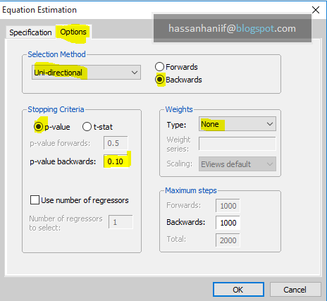
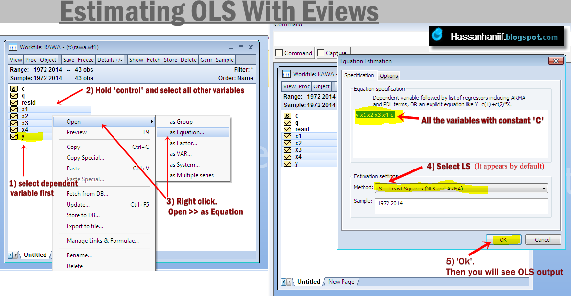
To estimate NARDL, follow these steps: 

Steps:
F

Step 1. Perform unit root tests to justify that non of the variables are I(2).

Step 2. Generate INFt+ and INFt–  from  INFt

Step 3. Run the Non linear ECM under NARDL

Step 4. Test the ‘non linear cointegration’ test with F-test

Step 5. check the asymmetries.

See my another post on estimating Nonlinear ARDL (NARDL) with Eviews.

NARDL With Eviews

Shin et al. (2104): 

Researchgate link
https://www.researchgate.net/publication/228275564_Modelling_Asymmetric_Cointegration_and_Dynamic_Multipliers_in_a_Nonlinear_ARDL_Framework


Some papers which applied NARDL:

1. Abdlaziz, Rizgar Abdlkarim, Khalid Abdul Rahim, and Peter Adamu. "Oil and Food Prices Co-integration Nexus for Indonesia: A Nonlinear ARDL Analysis." International Journal of Energy Economics and Policy 6.1 (2016).
2. Ndoricimpa, Arcade. "Analysis of asymmetries in the nexus among energy use, pollution emissions and real output in South Africa." Energy (2017).
3. Zhang, Zan, Su-Ling Tsai, and Tsangyao Chang. "New Evidence of Interest Rate Pass-through in Taiwan: A Nonlinear Autoregressive Distributed Lag Model." Global Economic Review (2017): 1-14.











References: 

1. Dufrénot, Gilles, and Valérie Mignon. Recent developments in nonlinear cointegration with applications to macroeconomics and finance. Springer Science & Business Media, 2012.  link

1.    Enders, Walter. Applied Econometric Time Series. Hoboken: Wiley, 2015. Print. 

1. Pesaran, M. Hashem, Yongcheol Shin, and Richard J. Smith. "Bounds testing approaches to the analysis of level relationships." Journal of applied econometrics 16.3 (2001): 289-326. link

1. Shin, Y., Yu, B., Greenwood-Nimmo, M.J., 2014. Modelling Asymmetric Cointegration and Dynamic Multipliers in a Nonlinear ARDL Framework. In William C. Horrace and Robin C. Sickles (Eds.), Festschrift in Honor of Peter Schmidt: Econometric Methods and Application, pp. 281-314. New York (NY): Springer Science & Business Media.  link

Eviews official website:

http://www.eviews.com/home.html 

Continue Reading...

Nonlinear ARDL (NARDL) Model With Eviews

Before you start reading, If you are not familiar with NARDL see A Quick Explanation of Recent NARDL where i formulated a food import model (for India for the illustration purpose). In this post, i estimated the NARDL model with Eviews 8/9.  The  raw data used to demonstrate with Eviews can be downloaded from google drive. Download Workfile. Or send a hi to my Email: hssanhanif@gmail.com or meet me at dept. of Economics and Banking, IIUC.  This file contains the yearly data of inflation rate and ''percentage of food import to total import'' of India . The food model has the following form: 

   Food_t=C+ INF_t+U_t

 Where, Food_t indicates % of Food Import of total import. (dependent variable) and  INF_t indicates inflation rate (independent variable).

Since NARDL is a recently developed model, Eviews 8, Eviews 9 or other current versions do not have any built-in option yet to estimate NARDL. So, 

Follow these steps:
F

Step 1. Perform unit root tests to make sure that non of the variables are I(2).

Step 2. Generate INFt+ and INFt–  from  INFt

Step 3. Run the Non linear ECM under NARDL

Step 4. Test the ‘non linear cointegration’ test with F-test

Step 5. check the asymmetries.

Step1: run unit root test to make sure that data are not I(2).

Like the ARDL error correction model by pesaran et al (2001), the NARDL does not allow I(2) variables. To perform unit root test in Eviews:  ⟾click on the series unit root test ⟾select level and ⟾select intercept and trend now see the p-value. If it is less than 0.05 the series is said to be ststionary or I(0) at 5% significance level. and if not repeat the steps and this time select the choice first difference. If p-value is less than 0.05 then series is said to be stationary at first difference or I(1). And if it is more than 0.05 the series is not I(1). And should not be entered in NARDL model. I have checked each series and found that Foodt is  integrated of order 1 or I(1) and inflation is found to be the integrated of order zero I(0).  So we can run NARDL. You can verify the order of integration with the Eviews workfile i provided in first paragraph. 

Step 2 Calculate partial sum of positive and negative change:

To do this, copy each line of the commands given in the box paste it into the command area of Eviews then press ENTER in keyboard. For example after putting  genr dinf = inf-inf(-1) press ENTER than put the 2nd line genr dfood=food-food(-1) then press ENTER and so on. To understand these commands, what  these commands to is that they create first difference variable of inf and food: dinf and dfood, then create a series for the values of dinf which are not negative and another  series for negatives. Then they calculate the cumulative sum of each after multiplying positive and negative series by the first difference. The resulting cumulative sums are partial sum of positive and negative changes in inflation, which denoted by inf_p and inf_n, respectively. 

Eviews Commands to decompose independent variable in NARDL.  Note: throughout this Eviews illustration,  INFt+ is denoted by inf_p and INFt– denoted by inf_n

genr dfood=food-food(-1) genr dinf = inf-inf(-1) genr pos = dinf >=0 genr dinf_p = pos*dinf genr dinf_n = (1-pos)*dinf genr inf_p = @cumsum(dinf_p) genr inf_n = @cumsum(dinf_n)

Eviews commands for decomposing a series into  partial sum of positive and negative change 

Step 3:  Run the Non linear ECM under NARDL 

 Step 3.1  Estimating NECM under NARDL framework

Now ⟾ click on quick estimate equation ⟾ choose two steps least square from drop down list and specify the equations in both of the boxes as shown the picture below. 

d(food) c food(-1) inf_p(-1) inf_n(-1) dfood(-1 to -4) dinf_p(-0 to -4) dinf_n(-0 to -4)

NARDL specification 

Explanation of the specification: The specifications in first box contains the dependent variable d(food), constant C, followed by 3 independent variables—the  first lagged term of food: food(-1),  the first lagged term of partial sum of positive change in inf which is denoted by inf_p(-1), and the first lagged term of partial sum of negative change in inf which is denoted by inf_n(-1). The second box contains the set of differenced variables upto 4 lags. ( i chose maximum lag 4 since the data are yearly). By specifying (-1 to -4), all the lagged terms of dfood from first lag to fourth lag are included. So as for the rest. 0 lag implies no lag. The 0 lag of Xt, for example,  is the Xt itself. Note here that the 0 lag is not included in case of dfood because dfood is already acting as dependet variable in the model. 

But, before you click OK, click ‘options’ and set the settings as shown in the picture below

This setting will drop the insignificant stationary variables from NARDL  model as suggested by Shin et al (2014)

Choose unidirectional, backwards, p-values, set p-value 0.10 (or 0.05 or even 0.01.) I chose 0.10 here. Also choose uni directional  and backwards.  The interpretation of this setting is that it will remove the variables that are not significat even at 10% level while it will retain the variables of upper panel of the box even if they are not significant this was chosen in shin' study. However, this setting is not hard and fast rule. The goal is to select the appropriate model specification with appropriate lags for the differenced regressors. You can choose other criteria to choose appropriate lags. 

3.B    NARDL output, long-run coefficients and interpretation: 

NARDL output in Eviews 

By a quick  glance to the output we can learn that Eviews removed some lags and that  0.308099 and 0.390456 are the coefficients of inf_p and inf_n, respectively. But they are not the long run coefficient. To calculate the long run coefficient divide the negative of coefficient of each inf_p and inf_n by the coiefficient of food(-1). So the long run coefficient of inf_p is -0.0308099 /-0.457567=0.673342  and long run coefficient of inf_n is -0.390456/-0.457567=0.853331 . clearly, both long-run coefficient are positive. hence So the long run equation or the cointegrating equation is :

            long run equation:        🔴   Food= 0.673342inf_p  + 0.853331inf_n +u

interpretation of NARDL output: 1 percent point increase in inflation rate leads to 0.67 percent point increase in food import India (positive realtion), and 1 percent point decrease in inflation rate leads to 0.85 percent point decrease in food import (also positive relation). (I said  percent point because the variables are rates) clearly, the food import response more to negative change because the coefficient is larger. 

Step 4: Asymmetric Cointegration test: 

Before drawing any conclusion regarding the estimated coefficients one needs to check if variables are co-inetgrated. The coefficients would be sporious if variables are not cointegrated.  For testing cointegration under NARDL, Shin at al recommended to use joint null hypothesis of level (non-diffrenced) variables and to compare the critical values of bound testing in pesran et al (2001). (You can download the paper from internet, and find the table in Page 300). If the calculated F statistics is found to be the greater than the upper critical value then there is evidence of co-integration. And if not, then evidence of cointegration is not found.

 To start cointegration test in Eviews click view on output window⟾coefficient diagonistics⟾wald test-coefficient restriction. ⟾Specify the restriction c(2)=c(3)=c(4)=0. Then click OK’. Clearly, this wald test perform the joint null hypothesis of the coefficient of food(-1) which is second coefficient in the list (hence the notation c(2)), and the coefficient of lnf_p which is c(3) and and the coefficient of inf_n which is c(4). Basically, this joint null hypothesis acts as the null hypothesis of no cointegration. The procedure is illustrated in the picture below. 

Asymmetric cointegration test under NARDL

After clicking OK you will see Wald test results as shown in the picture below.

The calculated F-statistics for this (asymmetric) cointegration test

The calculated F-statistics is 13.34022. now lets compare it with critical values of 

pesaran et al (2001).  Here is the screenshot. Of case III.  

Pesaran et al. (2001) critical values Case III. 

Case III was chosen because in the NARDL representation on my food model there is a constant.(intercept was not restricted). In the table, k denotes the number of long run regressors.  Note here that there are two independent variables in long run equation of my food model :inf_p and inf_n.  but I chose k=1. The reason is that, the variables actually came from from 1 variable, hence, the k lies between 1 and 2. Also notice in table that the critical value for small k is larger. If the null hypothesis of no cointegration is rejected by critical value of its smaller k, then according to shin et al(2014) there is a strong evidence of co-integration. In my food model i chose  k=1, but for large number of variables set k equal to number of regressors before decomposition. 

Decision: since The calculated F statisics is larger than  The crticical value 7.84 at 1% significance level, there is strong evidence of cointegration at 1% significance level. 

Step 5. Testing the presence of  asymmetry: 

both of the positive change and the negative change have the long-run positive effect on food import. But are they really (statically) different ?  an asymmetry test basically test if the coefficient are equal or not. If they are equal then threre is no asymmetry and if they are not then threre is evidence of asymmetry. Recall from step 3 .2 that we calculated long run coefiicient for inf_p and inf_n by –c(3)/c(2) and –c(4)/c(2), respectively.  So, To test the long run  asymmetry in Eviews click on wald test and write this command below in the restriction box of wald-test.

–c(3)/c(2)=–c(4)/c(2)

Eviews will show the wald-test results as in the picture below. 

Wald test results for asymmetry test. 

Decision:  Clearly, the null of hypothesis of equality is rejected as p-value is less than 0.05. Wald test indicates that there is asymmetry in the long run impact of inflation on food import in India.

The Last step: 

Check the robustness by various diagnostic tests. I will not explain theme here but I saved the results of what I have shown above including the results of diagnostic tests. If you are stuck please do not hesitate to ask me. 

Important Note: This is not a full fledged research, rather an illustration to show how to estimate NARDL.  This model may suffer from omitted variable bias or any type of model misspecification, I'm not claiming that these results are valid for India. 




Acknowledgement: 

I'm thankful to M.J. Greenwood-Nimmo, one of the author of Shin et al (2014),  and to Rizgar Abdlkarim, co-author "Oil and Food Prices Co-integration Nexus for Indonesia: A Nonlinear ARDL Analysis." International Journal of Energy Economics and Policy 6.1 (2016).

Eviews official website:
http://www.eviews.com/home.html 

Continue Reading...

Summary Statistics With Eviews

Continue Reading...

How to Estimate OLS with Eviews : Easy Steps

Continue Reading...

A Brief Interpretation of Output of Simple Regression

(1)

number of observations:  It must be greater than the 'number of

Number of variables plus 1'. Here we want to estimate for 1 variable only, so number of observations must be 3 or more , and we have 41 observations it is good.

 It is better to have Large number of observations to get a good result. (like 100 or more observations. (The larger the better )

(2) and (3)

C is the constant and its value is 0.155798. This result says that if there is no X, or say if X is zero then, value of Y is 0.155798.

(4)

0.422690 is standard error of 0.155798. Standard error measures how reliable the coefficient 0.155798 is. you can perform hypothesis test for 0.155798 and confidence interval with this value later. (The smaller the better)

(5)

 0.368588 is t-Stattistic for coefficient 0.155798

 If you divide coefficient by its standard error  you will get  its t-statistic.  0.155798/0.422690=0.368588. So 0.368588 is the t-Stattistics for 0.155798

T statistics tells us whether coefficient is significant or not. If  absolute t-statistics (without positive or negative sign) is greater than the critical value of T distribution then coefficient is significant. Insignificant otherwise. For instance, t-critical value for 41 observations and two parameters is 1.685 . since 0.368588 is not greater than 1.685 the coefficient 0.155798 is not significant.  However, for now  you don’t need to perform tests using t-statistics  because Eviews calculates P-values for you which is easier to calculate the significance .

(6)

0.7144  is P-value of t-Statistics

It tells us whether the coefficient is significant or not. It is easier than the (5) If P-value is 0.01 or smaller than 0.01 then, coefficient is significant at 1% level meaning that the estimated coefficient is very strongly significant. And if it is 0.05 or smaller than 0.05 than the coefficient is also strongly significant at 5% level. If it is  0.10 or smaller, then, the coefficient is significant but not so strong as previous two. In the table P-value is 0.7144 which means that the of 0.155798 is not significant. 

(7)

X is independent variable, the variable whose effect on Y you want to test

(8)

The coefficient for the independent variable. It is the most important part of this table. It tells us how much the dependent variable change if the X change 1 unit. The estimated value 1.025555 means that if X increase by 1 unit the Y increases by 1.025555 unit and if X decreases by 1 unit the Y decreases by 1.025555 unit. Please note, the coefficient is positive  it means the relation between X and Y is positive or X has a positive effect on Y . If you find a negative value then it means they have a negative relation or X has negative impact on Y.

(9) standard error for 1.025555. same explanation as (4)

(10) T-statistics for 1.025555. same explanation as (5)

(11) P-value of T-statistics (1.025555) same explanation as (6)

 note, here P-value is 0.0000 this is smaller than 0.01. it implies that the the  coefficient 1.025555 is strongly significant (at 1% significant level). Now you can say variable X  significantly affects Y, or Variable X has a statistically significant effect on Y.

(12) R-squared :

 It is always between 0 and 1 and generally positive. It tells you how much successful your model is in predicting . A  higher  R-square is better. In very poor model R square is close to zero like 0.03 etc. R-squared  is found to be   0.79193. it implies that  about 79% of changes in Y are explained by the changes in independent variable X.

(13) Adjusted r square :

It is always equal to or smaller than  the R-squared. It does the same job as R-squared does, measuring how much good your model is in predicting.  But it has a Specialty , that is, if you add more variable even irrelevant  variable  R squre  incresase  but adjusted r squae  doesn’t. Therefore adjusted R square is kind of smarter than the R square ;)   

The higher the  adjusted r square   (close to 1)  the better the model. Sometimes  in a very poor model adjusted R-square become negative . A negative r square is considered as zero r square .

(14) and (14) S.E. of regression and  Sum squared resid. :

Both measure how much the estimated Y differ from actual Y ( actual Ys  are the value of Y in Y series of your data file). Of course, you know, it is not good if they differ too far from each other. A smaller S.E. of regression and  a smaller Sum squared resid are the better for any model.

Note: S.E. of regression  is calculated by dividing the Sum squared resid  with df hence, In a regression with very large number of observation  S.E. of regression become very small.

(15) Log likelihood:

 It is useful when you compare two nested models. You’ll always find this value negative.  a higher value is better for example -40 is better than -90. A negative value but closer to zero  indicates a best fitting model. And you will choose a model  from two models that has a higher log-likelihood.

(16)  F-statistic :

 It is used for testing the overall significance of a model specially in a model where independent variables are more than one.  Do all the independent variables in the model significantly affect  the dependent variable ? F-statistics will answer this question.  If F-statistics  is greater than the F-critical then you can say that all the variables are significant . (the F-critical  values are available in last pages of Econometrics and Statistics books)

(17) Prob(F-statistic):

However you don’t need to check F-statistic and F-critical value. By looking  to the Prob(F-statistic) you can easily check overall significance of all independent variables. If the Prob(F-statistic) is equal or smaller than 0.01 you can say that all the variables jointly in the model  significantly affect dependent variable at 1% significance level.  If it is equal or smaller than 0.05 you can say that all the variables jointly in the model  significantly affect the dependent variable at 5% significance level. And if it is equal to or smaller than 0.10 this time you   can say that all the variables jointly in the model are significantly affect dependent variable at 10% significance level.

(18) Mean dependent var:

simply it is the average of Y the dependent variable.

(19) S.D. dependent var :

it measures how much the  values of Y differe from its average value.

(20)Akaike info criterion    (21)Schwarz criterion    (22)Hannan-Quinn criter :

They are calculated with almost same formulas using log-likelihood and are called MODEL SELECTION CRITERIA. Smaller values are preferred. If you have different models to compare, A preferred model is the model with smaller value of  (AIC), (SC) and (HQ) or with smaller value of any two of them.  However AIC  is best used for Time series models.

(24)  Durbin-Watson stat:

 It tells us whether our model suffer ‘serial correlation problem’

If it is  close to 2  ; No serial correlation in the model

If it is close to 0 ; positive correlation in the model

If it is close to 4 ; Negative correlation in the model

It is better if we get the Durbin-Watson stat near to 2 such as 1.70, 2.01, 2.20 etc.   In our model we found 1.69882 indicating no serial correlation in the model.

Important Note !
The purpose of this post is to give the basic idea about the results of a simple regression model computed by Econometric software. (I have used Eviews). So, some of my comments about some results are too straightforward. For example a ''higher R-square is better'' does not make sense if you are dealing with non-stationary variables.

Continue Reading...